Linear Regression: A Gentle Introduction

What is it?

The equation for linear regression is :

where :

• $y$ is the dependent variable, the variable we are trying to predict
• $x_i$ is the independent variable, the features our model is trying to use
• $\alpha_i$ is the coefficient (or weights) of our linear regression, they are what we are learning essentially
• $\epsilon$ is the error in our model

What we mainly try to do is try to fit the model. By fitting we mean, we need to find the set of coefficients that will form the best predictions for $y$, closest to the actual values. Finally it will be as easy as just plugging in the values of $x_i$ in the equation below to find your prediction

Assumptions of Regression Models

While making a regression model, one must always keep in mind the 4 rules that are assumed to be true before we move on to make the model!

Linear Relationship

The fundamental principle of multiple linear regression is that there is a linear relationship between the dependent (outcome) variable and the independent variables. This linearity can be visually assessed using scatterplots, which should indicate a straight-line relationship rather than a curvilinear one.

Edit: However, it is essential to clarify that while the relationship between the dependent and independent variables must be linear in terms of the coefficients, this does not preclude the need for transformations if the raw data exhibits non-linear patterns. It is specifically the relationship between the dependent variable and the model parameters, and not necessarily to the raw data itself.

Multivariate Normality

The analysis presumes that the residuals (the differences between observed and predicted values) follow a normal distribution. This assumption can be evaluated by inspecting histograms or Q-Q plots of the residuals, or through statistical tests like the Kolmogorov-Smirnov test.

Absence of Multicollinearity

It is crucial that the independent variables are not excessively correlated with one another, a situation referred to as multicollinearity. This can be assessed using:

• Correlation Matrices: Ideally, correlation coefficients should be below 0.80.
• Variance Inflation Factor (VIF): VIF values exceeding 10 suggest significant multicollinearity. Potential solutions include centering the data (subtracting the mean from each observation) or removing the variables contributing to multicollinearity.

Homoscedasticity

The variance of error terms (residuals) should remain consistent across all levels of the independent variables. A scatterplot of residuals against predicted values should not reveal any identifiable patterns, such as a cone-shaped distribution, which would indicate heteroscedasticity. To address heteroscedasticity, one might consider data transformation or incorporating a quadratic term into the model.

What happens if any one assumption fails?

Don’t worry, your main task to make a model that closely mimics the original data. If your model fails to do that, then closely see which assumption is failing and try to address it. Maybe try to add new data, augment some data, and try out different techniques such that your assumptions work out!

Extra Info : Slope and Intercepts

In the world of regression analysis, the slope is like the crystal ball of your equation. It tells you how much your dependent variable ($y$) is likely to change when your independent variable ($x$) increases. It can be found out by the below two formulas :

in the second formula, $r$ is the correlation co-efficient. $S_y$ and $S_x$ is the standard deviation of $x$ and $y$, and $r$ can be calculated as

In the world of regression analysis, the y-intercept is like the starting point of our story. Mathematically speaking, it’s the point where our regression line crosses the y-axis. In other words, it’s the value of $y$ when $x$ is zero. Here $m$ is the slope and $b$ is the y-intercept (note: the text incorrectly labels $m$ as slope in the first equation below, which is a repeat of the slope formula).

How does it work?

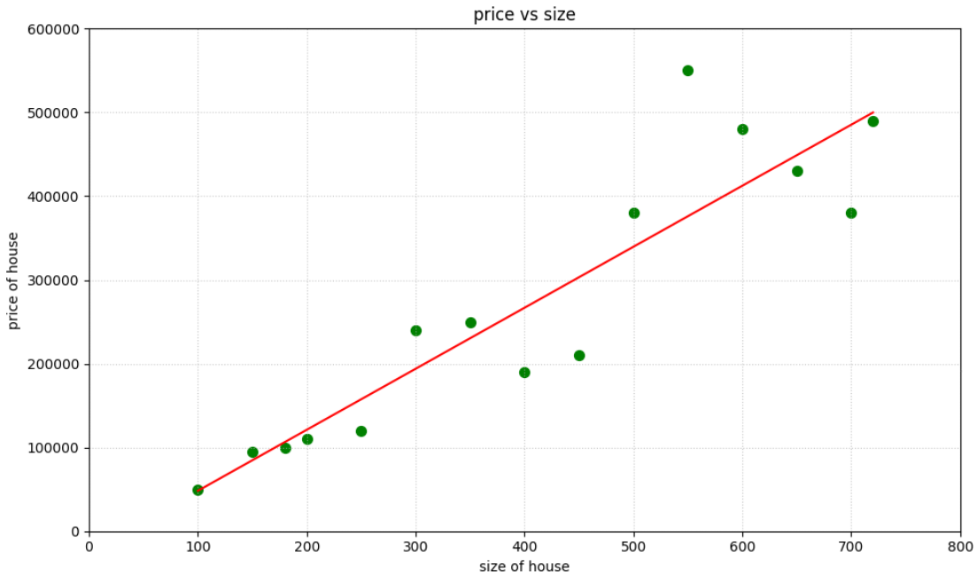
To actually understand how linear regression works, let’s try out an example. Let’s try to make a model that will predict the price of a house using the size of the house (in sqft)

It has exactly one feature, i.e the size of the house, so our linear regression equation will look like :

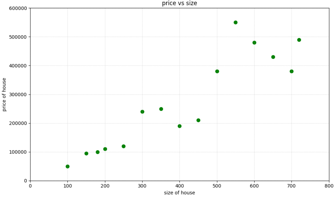
Let us first think of the most obvious answer for the model to be the average of this data $\sim$ 271666$

The equation becomes :

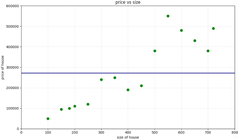
We can obviously see this model is very absurd as it will never predict the correct values for most of the input values. But we now need to know exactly how bad the model is. To find how our model works performance wise, we plot the error of each of our values. Error is nothing but the distance from the our original observation to our predicted observation.

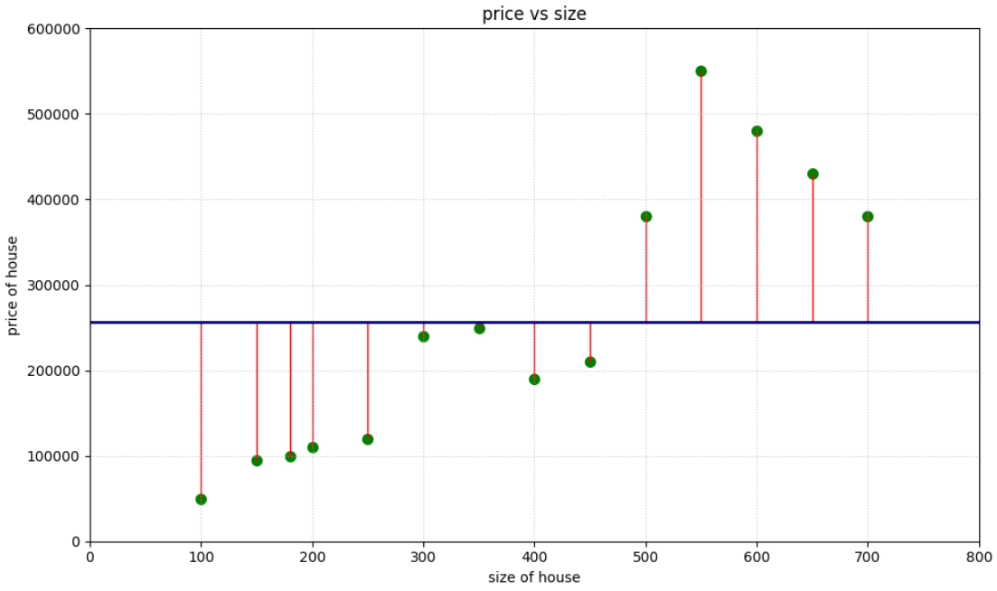
The main goal is to reduce this so that we find a line that fits our data the best! So basically we have to find the best possible values for $\alpha_1$ and $\alpha_0$. So here our main goal becomes to minimize something called the cost function

Cost Function

It is the function that measures the performance of a model. It in its essence is the calculation of the error between the predicted value and the expected values.

one common mistake

• cost function is the average of errors over $n$ samples of data
• loss function is the error for an individual data point

The cost function of a linear regression is nothing but Mean Squared Error, which is :

It works by squaring the distance between every data point and its corresponding point on the regression line

How to Minimize

We will be using the Gradient Descent algorithm which starts with some initial $\theta$ and repeatedly performs an update to find the minimum value of $J$. ($n=2$ according to our example)

First let’s try to solve the partial derivative term of the gradient descent algorithm for any single case of $(x,y)$

So the update rule becomes :

This rule of updatation is also called Widrow-Hoff Learning Rule. The magnitude of the update is proportional to the error term.

Normal Form

Now let’s try to find the $\theta$ that minimizes $J$. First we design a matrix $X$, with all the training examples and a $\vec{y}$, which will have all the target values from training set:

We can further show two results

Result 1

Result 2

To minimise $J$, we must find it’s derivative w.r.t to $\theta$

Hence for $J$ to be minimum, our $\nabla_\theta J$ has be to be $0$.

Hence, the value of $\theta$ that minimizes $J$ is given in closed form by the above equation!

The code for Linear Regression

Gradient Descent

def gradient_descent(X, y, learning_rate=0.01, iterations=1000):
    m, n = X.shape
    theta = np.zeros(n)
    for _ in range(iterations):
        h = X.dot(theta)
        gradient = (1/m) * X.T.dot(h - y)
        theta -= learning_rate * gradient
    return theta

Normal Form

def normal_equation(X, y):
    return np.linalg.inv(X.T.dot(X)).dot(X.T).dot(y)

Finally after applying all these logic, we find the equation to be